A Neural Network in the Browser

Table of Contents

1. User Manual
   1. Neural Network
   2. Playground
   3. Create own Datasets
2. Ready-To-Use Datasets
3. Implemented Elements
   1. Optimizers
   2. Losses
   3. Activation Functions
   4. Bias
4. Bibliography
5. List of Abbreviations

1.  User Manual

The purpose of this chapter is to outline how to use the learning software to build a neural network, train it and make predictions with it.

First: Build the Neural Network

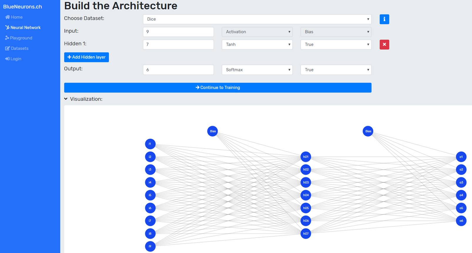
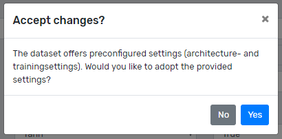
In order to build the neural network, the training dataset must first be selected. This can be achieved by selecting the desired dataset from the dataset dropdown. If preconfigured settings such as the architecture, the training settings or both are provided by a dataset, the user is asked whether he wants to adopt them (as can be seen in Figure 2). If the user clicks yes, the supplied architecture will be adopted, otherwise the currently entered architecture will remain.

The information about the dataset, such as the number of input neurons, output neurons, etc. can be obtained by clicking on the info button next to the dataset dropdown. The number of input and output neurons of the neural network must correspond to the values described in the dataset info. Otherwise the transition to the training page is blocked and a message is displayed. For each layer the number of neurons, the activation function and the bias can be selected. Hidden layers can be added via the button "+ Add Hidden Layer". Each hidden layer can be removed with the red button "x" at the end of the layer line. The visualization of the neural network is updated immediately after each input.

For each layer the number of neurons, the activation function and the bias can be selected. Hidden layers can be added via the button "+ Add Hidden Layer". Each hidden layer can be removed with the red button "x" at the end of the layer line. The visualization of the neural network is updated immediately after each input.

Second: Train the Neural Network

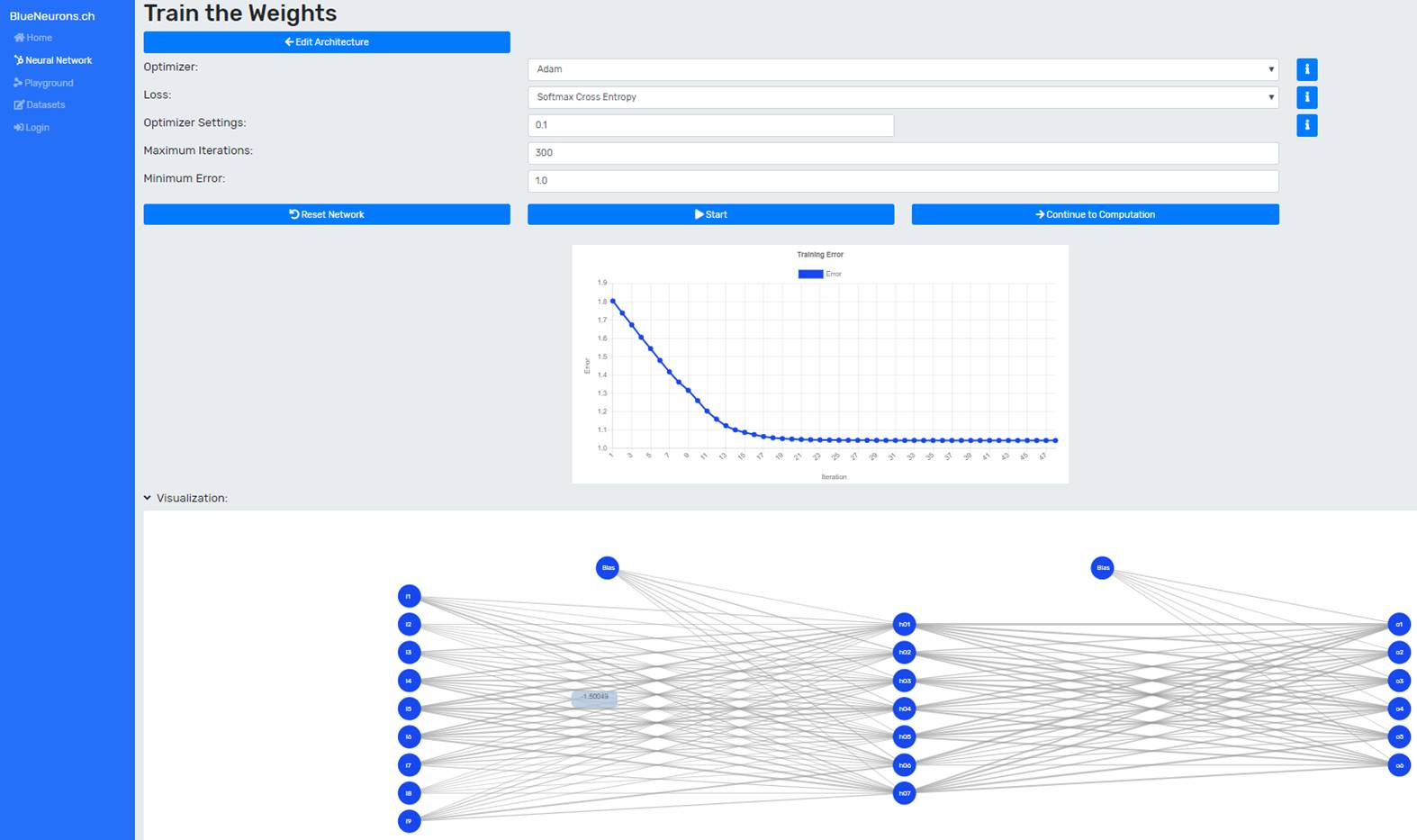
After the architecture was successfully built, the user can continue to train the neuronal network by pressing the button "Continue to Training”. The selected dataset can again contain predefined values for the training. If this is the case, these values are automatically taken over if the user has previously accepted to adopt the settings from the dataset. Otherwise, or if the dataset has no preconfigured training settings, the values must be selected manually.

First, an optimizer must be selected. The goal of an optimizer is to minimize the loss function. The user can choose between the stochastic gradient descent (SGD), SGD-Momentum, Adam and RMSprop optimizer.

The next step is to select the loss function. The user can choose between the mean squared error (MSE) and the Softmax cross entropy. The MSE is mostly used for regressions and cross entropy for classifications.

Now, depending on the chosen optimizer, the optimizer settings learning rate and momentum must be set. The learning rate allows the user to specify what percentage of the weight change the learning process should adopt. For example, if a learning rate of 0.2 is specified and the weight change is 0.4, the actual weight change will be 0.08. If the learning rate is too high, the minimum of the loss function will be overshot. If the learning rate is too low, the training will take extremely long or will get stuck. Momentum, which can be set with the RMSprop and SGD-Momentum optimizer, specifies how much of the previous weight change is added to the current weight change. This helps to accelerate the learning and improves the accuracy as it gives a bias for the direction of the gradient.

After the optimizer settings, the abort conditions must be set. The number of maximum iterations indicates how many training iterations will be performed before the training is aborted. The minimum error indicates the error value at which the neural network should stop the training.

Now the training can be started by clicking on the "Train" button. The error is now displayed in real time per iteration in the line diagram (see Figure 3). The "Reset Network" button distributes new initial weights to the network. This should be done especially if the training was not successful.

After training, the button "Continue without Training" has changed to "Continue to Computation". Clicking this button displays the calculation page.

Last: Make Predictions with the Trained Neural Network

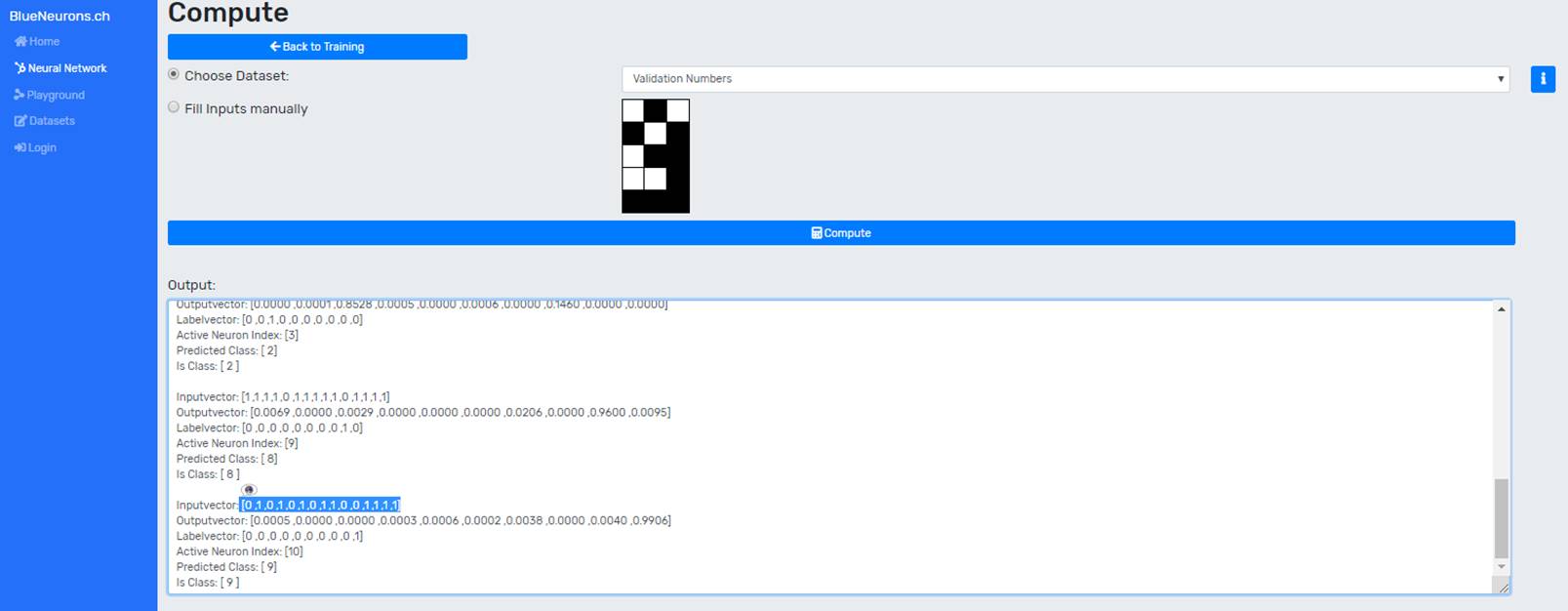
Depending on the dataset a validation set is supplied. Manual entries can also be made either via a drawing grid (if the dataset supports it) or via text fields. The preferred dataset can be selected via the dropdown. After selecting the dataset, the user can click on the "Compute" button to make a prediction for the whole dataset. Figure 4 shows the output console displaying the accuracy and calculation results of each item in the dataset:

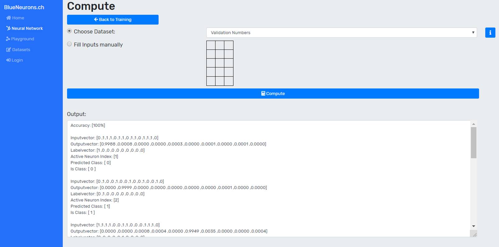
For accuracy calculations, the number of correctly classified elements is divided by the number of all classified elements. An element is considered as correctly classified if the index of the output neuron with the highest value corresponds to the index of the is-class in the label. For regressions, the mean squared error is calculated.

The input vector can be selected in order to display it in the drawing grid (as can be seen in Figure 5).

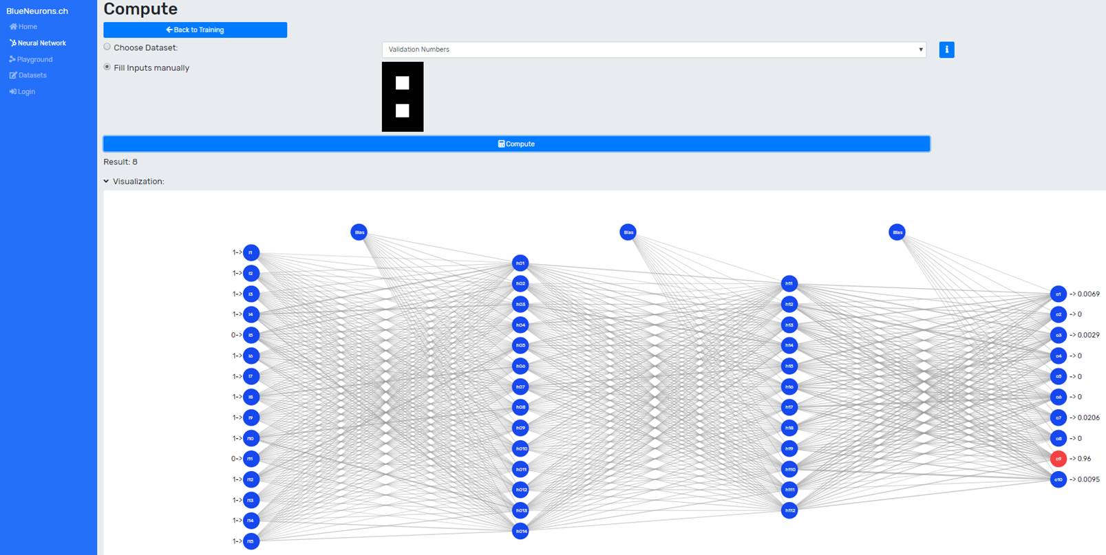
The mode can be switched to "Fill Inputs manually" to draw and classify own drawn elements. The desired element can be drawn by clicking on the individual cells in the drawing grid. The next step is to press the "Calculate" button. The result is displayed as text below the button and in a visualized form. In the visualization of the neural network the input values and the output values can be seen. The neuron with the highest output value is marked red (it fires the most) and thus represents the predicted class. Since the first neuron represents class 0 and the last neurons class 9, the drawn number was correctly predicted as 8.

1.2  Neural Network Playground

The playground demonstrates the relationship between the various settings of a Neural Network (e.g. activation function, weights, input values and bias) and the resulting output value. Changes are immediately displayed in the visualization of the Neural Network.

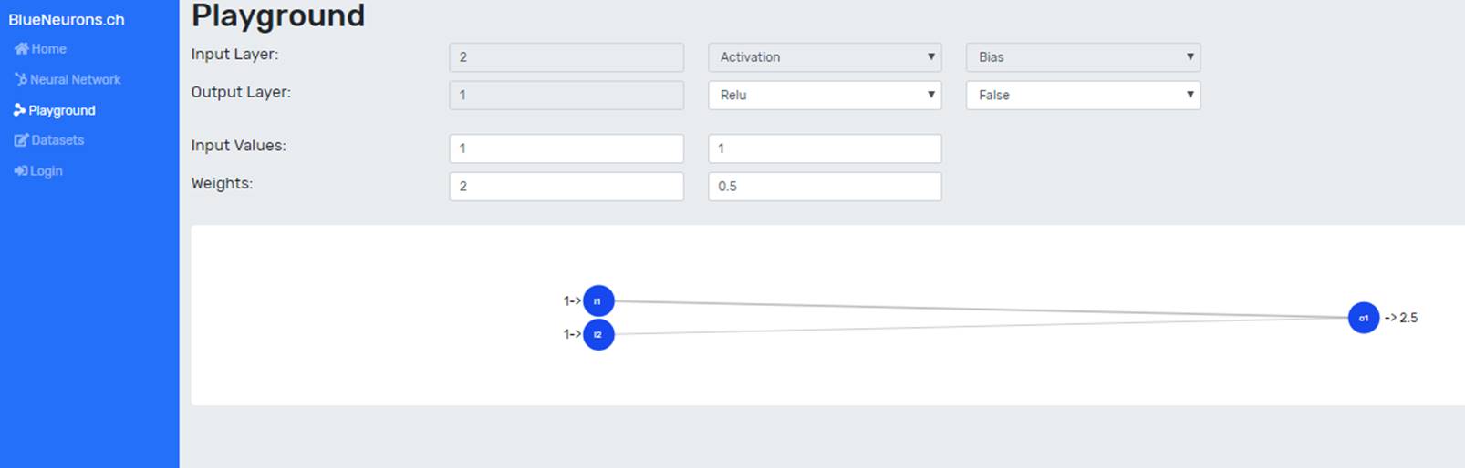
When the binary step function is selected, an additional line is displayed in which the weights can be automatically adjusted to solve the OR problem. In order to run the algorithm, a learning rate between 0 and 1 must be specified and the button "Perform one Training Epoch ('OR'-Problem)" must be clicked. After each epoch, the weights will be adjusted automatically. Depending on the selected initial weights and learning rate, fewer or more epochs are necessary. As soon as the weights are no longer adjusted by the algorithm, the weights are optimized so that the perceptron is able to solve the OR problem.

1.3  Create your own Datasets and use it in the Neural Network Software

In the dataset editor, existing datasets can be viewed or new ones can be created. Existing datasets can be selected via the dataset dropdown. A new dataset can be created by selecting “Create new Dataset” in the dropdown.

When creating a dataset, a unique name and publication type must first be chosen. With "public" the dataset is available to all users, with "private" only to the creator as long as he is logged in. Now the dataset can be created in JSON-format using the JSON-editor, whereby the following attributes exist:

• description: (String) A description of your dataset.
• isValidationset:(Boolean) Specifies whether the dataset may only be used for validation purposes and not for training purposes.
• problemType: (String) Choose between "classification" and "regression".
• items: Represents an array of items with the following attributes:
  • data: (Float array) Represents the data of the item.
  • labels: (Float array) Represents the result for the entry (for classification use one-hot encoding).
• matrix (optional): (Int array with length 2) The first entry specifies the number of rows and the second entry the number of columns of the drawing matrix. As soon as a matrix is defined, the "Vector Helper" is displayed at the bottom. With the "Vector Helper" the input vectors can be created using the drawing grid.
• outputDescription (optional, for classifications only): (String array) Represents a description for each output neuron. For two output neurons where the first one represents false and the second one true, you would enter the following:

• "outputDescription": [

      "False",

      "True"

    ]

• layers (optional): A predefined architecture for the neural network can be provided here. It represents a layer array where the first entry is the input and the last entry is the output layer. For the input layer only the number of neurons has to be specified, for the other layers the number of neurons, the activation function and the bias have to be defined. A layer has the following attributes:
  • neurons: (Int) Number of neurons
  • activation: (String) Choose between "relu", "tanh", "sigmoid" and "softmax".
  • bias: (Boolean)
• trainingSettings (optional): Predefined settings for the training can be made here with the help of the following attributes:
  • optimizer: (String) Choose between "sgd" (stochastic gradient descent), "sgdm" (stochastic gradient descent with momentum), "adam" or "rmsprop".
  • loss: (String) Choose between "mse" (mean squared error) and "sce" (softmax cross entropy).
  • learningRate: (Float) Learning rate
  • momentum: (Float) Momentum (only with optimizers RMSprop and SGDM)
  • maxIterations: (Int) Maximum iterations before the training is aborted.
  • minError: (Float) When this error value is reached, the training stops.

After all values have been defined, press the save button. The dataset should now be saved and visible in the dataset list if all values have been correctly defined. If a value has not been configured correctly, an error message will be displayed.

2  Ready-To-Use Datasets

All datasets provided in the learning software have a predefined architecture and well operating training settings. The following datasets are included in the learning software:

OR-Dataset

The OR-problem represents a linear problem and can therefore be solved with an Single-Layer-Perceptron (SLP).

XOR-Dataset

The XOR-problem represents a non-linear problem and therefore an MLP is required to solve it.

Dice-Dataset

The dice dataset represents the six eyes of a dice. It can be used together with the drawing grid to draw the eyes of the dice.

Numbers-Dataset

The numbers dataset represents the numbers from 0 to 9. It can be used together with the drawing grid to draw different numbers. This dataset is complex to train because different spellings were used and the distribution of the numbers is uneven. For example, there are more different spellings for the number 1 than for the number 8. In order to evaluate the Neural Network, a validation set has been provided. If the accuracy for the validation set is not sufficient (e.g. < 100%), it is recommended to go back to the training page, reset the network (new initial weights are distributed), adjust the parameters when necessary and to train the Neural Network anew.

Letters-Dataset

The letters dataset contains all letters from A to Z. It can be used together with the drawing grid to draw different letters. This dataset still has a lot of potential, because many more variations of letters can be added. A validation set is also available for this dataset, but due to the few variations of the letter spellings in the training set it is almost impossible to achieve 100% accuracy on the validation set.

3  Implemented Elements in the Neural Network Learning Software

In this chapter the implemented elements of the learning software will be introduced.

3.1  Optimizers

There are various optimization algorithms that can be used in order to minimize the error/loss function (Walia, 2017b). The following optimizers are implemented in the learning software:

Stochastic Gradient Descent

The following paragraph is based on Bergen, Chavez, Ioannidis and Schmit (2015, pp. 1-2).

Stochastic gradient descent (SGD) is a popular optimization method in machine learning. The method is based on the idea that at each iteration a data element is selected randomly and that the gradient of the entire dataset can be estimated due to this element. The advantage of this approach is that it is not necessary to go through the entire dataset in order to calculate the gradient. However, this method needs more iterations to converge, since the training is very noisy due to the estimation.

Parameter: Learning rate (required)

Stochastic Gradient Descent with Momentum (SGDM)

Momentum adds a fraction of the past weight change to the current weight change and therefore helps SGD to find the right direction towards a minimum (Ruder, 2016, p.4). Bushaev (2017) claims that this technique can lead to a better estimation of the actual gradient than the classic SGD without momentum. Parameters: Learning rate (required) and momentum (required)

Adaptive Learning Rate Optimizers (RMSprop and Adam)

The following paragraph is based on Moreira and Fiesler (1995, pp. 1-3).

With SGD and SGDM, the learning rate defined at the beginning always remains the same. However, it has been shown that an appropriate adjustment of the learning rate during training has a positive impact on the result. In the area close to the minimum it is desirable to have a small learning rate. If the minimum is further away, a larger learning rate is better to accelerate the training. Another advantage of adaptive learning rate optimizer is that the trial-and-error search for the optimal parameters can be avoided (Moreira & Fiesler, 1995). For these reasons, in addition to the static learning rate optimizers, two adaptive learning rate optimizers have been added:

Adam

Parameter: Initial learning rate (optional)

RMSprop

Parameters: Initial learning rate (required), momentum (optional)

Ruder (2016) claims that Adam and RMSprop are very similar. However, he also mentions Kingma and Ba (2015, pp. 5-8) who show some important differences between the two, resulting in Adam outperforming RMSprop in the tests they performed. Nevertheless, both optimization methods were added in order to make a direct comparison possible.

3.2  Losses

A loss function measures how well a neural network performs. The goal of training a neural network is to minimize the loss function (Sosnovshchenko, 2018; Walia, 2017b). Two loss functions covering regression and classification tasks were implemented in the learning software:

Mean Squared Error

The mean squared error (MSE) is a popular loss function for regression problems (Grover, 2018; Sosnovshchenko, 2018). It measures the quality of an estimator by calculating the average squared distances between the estimated points ỹ and actual points y (Zheng, 2013):

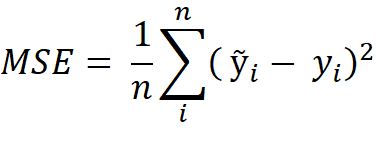
• n: Number of all estimates
• i: Index of current estimate

Softmax Cross Entropy

The following paragraph is based on Gomez (2018):

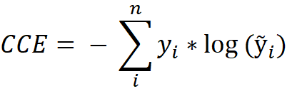
Softmax Cross Entropy (SCE), also known as categorical cross entropy (CCE), is used for multi-class classification problems. The label vector of an element must be one-hot encoded, which means that only one class in the vector can be active (Gomez, 2018). The CCE is defined in the equation below, where y is the label vector, ỹ is the output vector for the element to be classified and n represents the length of both vectors, respectively the number of classes (Sosnovshchenko, 2018):

Example:

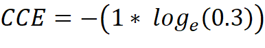
If a dataset with pictures of dogs, cats and horses is present, the one-hot encoded label vector has a length of 3, because it must represent three classes [dog, cat, horse]. When training the neural network, a data element which represents a cat is pulled and therefore has the following label vector [0, 1, 0]. The untrained neural network gives us the output vector [0.2, 0.3, 0.5] which expresses the predicted probability of each class for the given data element. Now the CCE can be calculated:

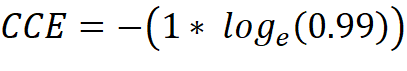
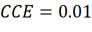
As the prediction gets better, the CCE gets smaller and is therefore suitable to calculate the loss of a classifier:

3.3  Activation Functions

An activation function calculates the output signal of the neuron based on the aggregated input signals (Tadeusiewicz et al., 2015, S.36). The output indicates if a neuron has fired or not (Nwankpa, Ijomah, Gachagan, & Marshall, 2018, S.3). Non-linear activation functions bring non-linear properties to an MLP (Nwankpa et. al., 2018, S.4; Walia, 2017a). According to Walia (2017a), Sigmoid, Tanh and ReLU are the most popular activation functions. In order to calculate the probability for multiclass problems, the Softmax activation function has been added. The linear and the binary step function were added at the request of the client.

Binary Step

The following explanation of the binary step function is based on Serengil (2017).

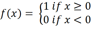
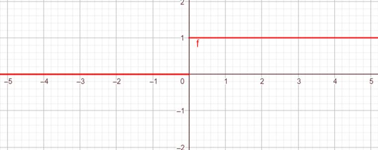
This activation function is called binary step function because it returns binary values, i.e. 0 or 1 (see Figure 8). It is mostly used in single layer perceptrons which can only classify linear problems. The problem with the binary step function is that in real world applications the backpropagation algorithm is used which requires differentiable activation functions. However, the derivative of the binary step function is zero and therefore the backpropagation algorithm cannot update the weights because any number multiplied by zero is always zero. For this reason, the binary step function can only be found in the playground and not in the neural network part of the learning software.

The binary step function is defined as follows:

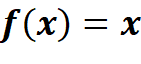
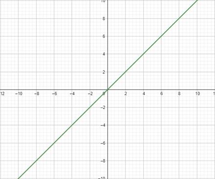
Linear

As can be seen in Figure 9, the output of the implemented linear activation function is the same as its input. Linear activation functions do not bring non-linear properties to an MLP. This means that e.g. the XOR-problem could not be solved by an MLP if only linear activation functions were used.

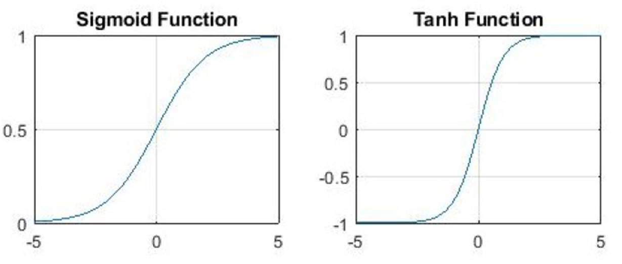
Sigmoid

The following paragraph is based on Nwankpa et. al. (2018, p.5).

The Sigmoid function, also known as logistic function, outputs a value in the range from 0 to 1 and can therefore be used in the output layer of a Neural Network to produce probability-based outputs. It is mostly used in binary classification problems whereas the Softmax activation function is used for multi-class classification problems.

Tangens Hyperbolicus (Tanh)

The Tanh function returns a value in the range from -1 to 1. LeCun, Bottou, Orr and Müller (1998, p.18) state that Tanh often converges faster than Sigmoid.

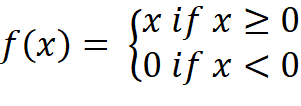
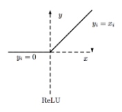
Rectified Linear Unit (ReLU)

The following paragraph is based on Nwankpa et. al. (2018, pp. 5-9).

ReLU is a popular activation function for deep neural networks. The advantage of ReLU over Sigmoid and Tanh is that ReLU does not have the problem of vanishing gradient when training deep networks. The problem with Sigmoid and Tanh is that the inputs are squeezed into a very narrow range between 0 and 1 and -1 and 1 respectively. Consequently, the derivation of the function is very small in certain places. When now training the Neural Network using backpropagation, the following problem arises: «With successive multiplication of this derivative terms, the value becomes smaller and smaller and tends to zero, thus the gradient vanishes» (Nwankpa et. al., 2018, p. 5). Therefore, ReLU should be used in hidden layers of deep networks.

ReLU is a nearly linear function f(x) which is defined as follows:

Softmax

The following paragraph is based on Nwankpa et. al. (2018, p.8).

The Softmax activation function outputs the probability for each given class in a vector. This means that each class is assigned with a value between 0 and 1 so that the sum of all classes in the output vector adds up to 1. Therefore, this activation function should be selected for the output layer when solving a multi-class classification problem.

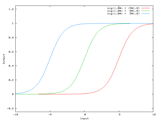
3.4  Bias

When configuring each layer of a Neural Network a bias can be selected in addition to the previously mentioned number of neurons and activation function. Solely for the input layer a bias is not set as its value would be overwritten by the input values. The bias always has a constant output, usually 1. The bias is fully connected to its associated layer and causes the activation function to move to the left or right (as can be seen in Figure 12), while the weights affect the slope of the activation function (Collis, 2017):

4  Bibliography

Bergen, K., Chavez, K., Ioannidis, A., & Schmit, S. (2015). Distributed Algorithms and Optimization, Spring 2015. Abgerufen von https://stanford.edu/~rezab/classes/cme323/S15/notes/lec11.pdf

Bushaev, V. (2017, Dezember 4). Stochastic Gradient Descent with momentum. Abgerufen 15. Mai 2019, von https://towardsdatascience.com/stochastic-gradient-descent-with-momentum-a84097641a5d

Collis, J. (2017, April 14). Glossary of Deep Learning: Bias. Abgerufen 27. April 2019, von https://medium.com/deeper-learning/glossary-of-deep-learning-bias-cf49d9c895e2

Gomez, R. (2018, Mai 23). Understanding Categorical Cross-Entropy Loss, Binary Cross-Entropy Loss, Softmax Loss, Logistic Loss, Focal Loss and all those confusing names. Abgerufen 16. Mai 2019, von https://gombru.github.io/2018/05/23/cross_entropy_loss/

Grover, P. (2018, Juni 5). 5 Regression Loss Functions All Machine Learners Should Know. Abgerufen 16. Mai 2019, von https://heartbeat.fritz.ai/5-regression-loss-functions-all-machine-learners-should-know-4fb140e9d4b0

Kingma, D. P., & Ba, J. (2015). Adam: A Method for Stochastic Optimization. ICLR 2015, 1–15. Abgerufen von http://arxiv.org/abs/1412.6980

LeCun, Y., Bottou, L., Orr, G., & Müller, K.-R. (1998). Efficient BackProp. In Neural Networks: Tricks of the Trade. New York: Springer Verlag.

Moreira, M., & Fiesler, E. (1995). Neural networks with adaptive learning rate and momentum terms. Abgerufen von https://www.uni-muenster.de/AMM/num/Vorlesungen/ Seminar_Wirth_Master_WS18_b/handouts/Plagwitz.pdf

Nwankpa, C., Ijomah, W., Gachagan, A., & Marshall, S. (2018). Activation Functions: Comparison of trends in Practice and Research for Deep Learning. Abgerufen von http://arxiv.org/abs/1811.03378

Ruder, S. (2016, Januar 19). An overview of gradient descent optimization algorithms. Abgerufen 16. Mai 2019, von http://ruder.io/optimizing-gradient-descent/index.html

Serengil, S. I. (2017, Mai 17). Step Function as a Neural Network Activation Function. Abgerufen 14. Juni 2019, von https://sefiks.com/2017/05/15/step-function-as-a-neural-network-activation-function/

Sosnovshchenko, A. (2018). Machine Learning with Swift. Birmingham: Packt Publishing Ltd.

Tadeusiewicz, R., Chaki, R., & Chaki, N. (2015). Exploring Neural Networks with C#. In Exploring Neural Networks with C#. Boca Raton: CRC Press.

Walia, A. S. (2017a, Mai 29). Activation functions and it’s types-Which is better? Abgerufen 26. April 2019, von https://towardsdatascience.com/activation-functions-and-its-types-which-is-better-a9a5310cc8f

Walia, A. S. (2017b, Juni 10). Types of Optimization Algorithms used in Neural Networks and Ways to Optimize Gradient Descent. Abgerufen 27. April 2019, von https://towardsdatascience.com/types-of-optimization-algorithms-used-in-neural-networks-and-ways-to-optimize-gradient-95ae5d39529f

Zheng, S. (2013). Methods of Evaluating Estimators. Abgerufen von http://people.missouristate.edu/songfengzheng/ Teaching/MTH541/Lecture notes/evaluation.pdf

5  List of Abbreviations

Abbreviation	Meaning
CCE	Categorical cross entropy
MLP	Multy-layer perceptron
MSE	Mean squared error
NN	Neural network
SCE	Softmax cross entropy
SLP	Single-layer perceptron